Alfonso Sánchez-Beato's blog – Programming, IoT, and some side projects

How to schedule meetings in the minimal number of time slots

Although I work for a mostly remote work company, a couple of times a year we meet together for a week in some nice location of the world. When that happens, multiple meetings across people in different teams are organized. Sometimes the number of requested sessions gets out of hands and the scheduling team is overwhelmed. Quoting them in one of our latest gatherings: “We currently have over 160 proposed breakout sessions which will be impossible to schedule unless we work until midnight every day! We only have 3-4 hours available for breakout sessions each day.”

The problem with scheduling these meetings is that you get a mix of people from different teams so you have incompatibilities between meetings, and some persons are invited to many meetings and it becomes hard to solve all of these conflicts so all the invited people can join their meetings. So, it seemed an interesting problem and I wondered if I could find a way to solve this in an automated way.

The way I thought about the problem was that I needed to assign meetings to time slots, minimizing the number of these slots while at the same time making sure that meetings at the same time slot were compatible.

The first approach one can think about is simple brute force: go across all possible options and select one that produces the minimal number of time slots (note that it is possible that there is more than one optimal solution). To find all combinatorial options, first we can create all possible sets containing a given number of meetings. If we have $N$ meetings, we can create all the $K$ possible sets of meetings by first making sets that contain only one meeting, which is ${N\choose 1}$, then creating all possible sets that contain two meetings, which is ${N\choose 2}$, and so on, having finally $K$ sets that is

\[K=\sum_{i=1}^N {N\choose i}\]

These sets could represent meetings that would happen at the same time slot. Of them, only the ones containing compatible meetings will be valid. Compatibility is easy to find out: if no meeting invitees for two meetings are shared, those meetings are compatible. We will call the number of valid meeting sets $K_c$. Once we have them we can create other sets that contain, similarly, all possible combinations of these meeting sets. We can call them time slot sets. All possible combinations would give us the number $L$:

\[L=\sum_{i=1}^{K_c} {K_c\choose i}\]

Each of these time slot sets represent possible solutions to the problem, being the cardinal of the set the number of time slots that would be needed. However, not all combinations of time slot sets will be valid solutions: only the ones where no meeting is repeated across its meeting sets while at the same time all meetings are present will be valid. Among those, the combinations that have a minimal cardinal will be optimal solutions we want to find.

This is a correct way of finding a solution, however the number of combinations that we need to explore when we have more than just a few meetings can be daunting. Assuming a very optimistically low $10\%$ of valid sets of meetings, so $K_c=0.1 K$, we would have for, say, number of meetings $N=5, 8$, and $10$ a number of sets of time slots $L=7, 3.36 \cdot 10^7$, and $ 5.07 \cdot 10^{30}$. We can see how the numbers grow extremely fast, and that searching through all of them would take a lot of time and computer memory and become unfeasible very quickly.

So, we really need something better than pure combinatorics. Something that can help with this sort of problem is to try to visualize it to obtain some insight on how it could be solved, and I followed that route. In this case we can use non-directed graphs in a straightforward way: we can make each meeting a node, and connect with edges compatible meetings. I will explain this with an example. Let’s say that we have 8 people to which we will assign letters A to H and they attend 8 different meeting with different attendees. Attendees per meeting are as shown in the following table:

Meeting 1	A, E
Meeting 2	B, F
Meeting 3	C, G
Meeting 4	D, H
Meeting 5	B, C, D
Meeting 6	A, C, D
Meeting 7	A, B, D
Meeting 8	A, B, C

From the table we can calculate the adjacency matrix of the graph, where each row will show the compatibility between a meeting and the others, having a $1$ if compatible or $0$ if incompatible. We will obtain a symmetric matrix. In our example:

\[A=\begin{bmatrix}0 & 1 & 1 & 1 & 1 & 0 & 0 & 0 \\
1 & 0 & 1 & 1 & 0 & 1 & 0 & 0 \\
1 & 1 & 0 & 1 & 0 & 0 & 1 & 0 \\
1 & 1 & 1 & 0 & 0 & 0 & 0 & 1 \\
1 & 0 & 0 & 0 & 0 & 0 & 0 & 0 \\
0 & 1 & 0 & 0 & 0 & 0 & 0 & 0 \\
0 & 0 & 1 & 0 & 0 & 0 & 0 & 0 \\
0 & 0 & 0 & 1 & 0 & 0 & 0 & 0
\end{bmatrix}\]

For instance, from the first row we see that meeting $1$ is compatible with meetings $2, 3, 4$ and $5$. The graph that would result from here is:

The problem is transformed now into trying to find out how to group nodes that are one edge away of each other in sets, in a way that minimizes the number of sets while all nodes are included in some set and there is no overlap across sets. These groups of nodes would be in a single time slot of the schedule, and we will call such sets simply “slots”. Possible slots for this example would be $\{1,5\}$, $\{1,2\}$, or $\{1,2,4\}$, but not, for instance, $\{1,2,5\}$ as $2$ and $5$ are incompatible.

Different strategies con be tried to create such sets. The one that gave me best results was what I called a “removal strategy”. We start with each node being assigned to a different slot, and then we try to remove the maximum number of slots. We do that by iterating on the slots and checking if it is possible to move all nodes inside a slot to other already existing slots. If that is the case, we assign the nodes to those slots and remove the slot that contained them. The iterations will repeat until there is a point in which it is not possible to remove more slots. In the previous example, a possible evolution would be (each color represents a different time slot):

1. Each node gets assigned its own slot, that we will designate by colors in the image.

2. We look at the “blue” slot. We find that its only node (1) can be assigned to other slots (“red”, “green”, “beige”, or “violet”). Arbitrarily, we assign node 1 to the “red” time slot and remove “blue”.

3. We look at the “beige” slot. We find that its only node (4) can be assigned to other slots (“red”, “green”, or “brown”). Arbitrarily, we assign node 4 to the “green” slot and remove “beige”. We then look at “violet”, but it is not removable because of the only connected slot, “red”, one of its nodes (2) is not compatible with 5. We go through “orange”, “yellow”, and “brown”, but we are in similar situations and they cannot be removed.

4. We look now at “red”. We see that its two nodes can be assigned to other slots (1 can be assigned to “violet” or “green”, 2 can be assigned to “orange” or “green”). Arbitrarily, we assign 1 to “violet” and 2 to “orange”, and we remove “red”.

5. We look now at “green”. We see that its two nodes can be assigned to other time slots. Arbitrarily, we assign 3 to “yellow” and 4 to “brown”, and we remove “green”. We start another iteration and look at the four remaining time slots, but we find that none of them can be removed as we cannot assign all its nodes to alternative slots. Therefore, the algorithm finishes at this point. We went down from 8 to 4 slots, each of one with two meetings.

We have find a solution in just two iterations, instead of having to go through millions of combinations!

I went forward with this idea and implemented it in go. The implementation is not complicated and can be found in this github repository, which also contains some instructions on how to run it. The program accepts input in CSV format and outputs CSV as well, so the data can be easily exported/imported from any spreadsheet. More details on the format can be found in the README.md file.

The complexity of the algorithm is $O(N^2)$ because of the calculation of the adjacency matrix, but the maximum number of iterations of the removal strategy is just $N$. Convergence is assured as you obviously cannot remove more than $N-1$ slots. However, the algorithm does not always find the optimal solution, as we can find counter examples for this. For instance, if by using the removal strategy we end up with the following graph (again colors represent slots):

Figure 6

We can see that the algorithm will not process further the graph (no slot can disappear by assigning nodes to others). But, this one graph:

Figure 7

does have less slots (5 vs 6). There are some things that I think could improve the algorithm though. The first idea I have is, instead of assigning arbitrarily nodes to other slots when we remove, we could choose the one with less nodes amongst the possibilities, so distribution is more “even”. The second would be to proceed to further optimizations after applying the algorithm once by selecting neighboring slots, and then assign where possible nodes from them to the rest of the slots. With the remaining nodes, proceed with the removal strategy, and check if some slot consolidation happen. If that’s the case we would end up with less slots that those selected first. Doing this with the graph from Fig. 5 would actually lead to Fig. 6 after applying these steps to the green and orange slots. However, I doubt that arriving to an optimal solution is guaranteed even with these changes.

To finalize, I applied the algorithm to the original problem that inspired this blog post, and I was able to squeeze 158 meetings in 22 time slots in a fraction of a second, in just 3 iterations (it was nice to see that the very fast convergence happens also in more complex cases than the example). So it turns out that assuming we could have 4 hours for these meetings per day, we would not have been able to organize the schedule without some conflicts… although for a very small margin!

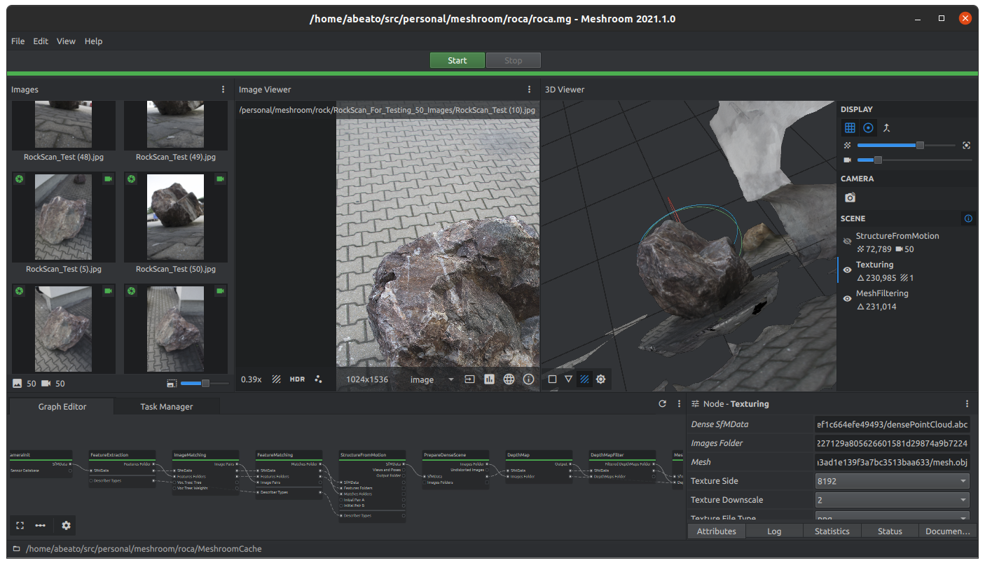
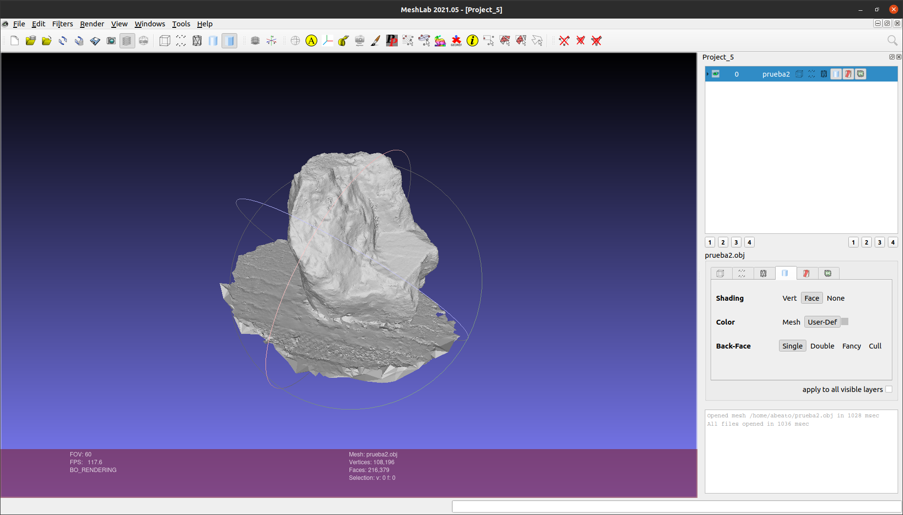
A MeshLab plugin to find optimal oriented bounding boxes

I have some interest in photogrammetry, and, more concretely, in the ways to extract 3D information from a set of photographies of an object. There is excellent open source software that is able to do this, like Meshroom, which is based on the Alice Vision framework. Once you create a 3D object with this tool, you have a set of vertices and textures that can be manipulated with specialized 3D editing software. And here again we have excellent open source software for this task, like MeshLab.

MeshLab can be extended via plugins, of which there is an extensive list. Some of them are integrated in the main MeshLab repository, but some others can be found in the MeshLab extra plugins repo. As I wanted to research what sort of measurements I could take on my 3D reconstructions, it looked like writing a MeshLab plugin was a great way to do this and be able to visualize and interact with the results easily.

I had some fun last year with finding optimal rectangles for videoconferences, so somewhat following that line of thought, I wondered how easy was to put an irregular object into an oriented bounding box (OBB) with minimal size, that is, the rectangular parallelepiped of minimal volume that encloses the object. This is called the optimal OBB in the literature. That seemed like a nice fit to try MeshLab plugins and learn how to do measurements on 3D reconstructions at the same time. Also, optimal OBBs have very important applications, such as fast rendering of 3D scenes, collision detection, and others. And optimal packaging might be an application as well indeed.

I put my hands on the task and started to dig into the literature on the topic. There is an exact algorithm to find optimal OBBs found by O’Rourke¹, but it is known to be slow (complexity is $O(N^3)$ being $N$ the number of vertices) and difficult to implement, so I looked at approximate algorithms. The one from Chang et al² looked fast and results were very near to O’Rourke’s solution. Also importantly, the authors published Matlab sources for it, so I chose that one for implementation in MeshLab. They called this algorithm HYBBRID because it mixes genetic algorithms with the Nelder-Mead optimization method, that can be used when derivatives for the target function cannot be calculated.

An OBB is defined by a rotation matrix $R$, the center of the box, and the size of each dimension. The most important part to obtain an optimal OBB is finding the rotation matrix, as once we have it it is trivial to calculate the other parameters by rotating the vertices with $R^T$ and then finding the minimum and maximum coordinates in the x, y, and z axis. Without digging too much into the details (I defer to the paper for that), the HYBBRID algorithm applies a genetic algorithm to sets of rotation matrices. With the ones that produce the smaller volumes, it applies the Nelder-Mead algorithm to find a local optimum. Finally, it applies a further refinement to the best solution by applying the 2D rotating calipers algorithm³ to each rotated axis. The genetic algorithm does a global sampling of the space of rotation matrices, while Nelder-Mead and 2D rotating calipers try to find a local minimum. The minimization function is not convex and not differentiable, although continuous, so this combination of algorithms works really well.

My C++ implementation for MeshLab has already been merged to the extra plugins repository, and can be found here (this was the original PR). I used the Matlab code as reference, with some improvements in the 2D calipers algorithm and in the calculation of average rotations. The filter adds two meshes to the object to which it is applied, one with the convex hull of the object and another one that defines the bounding box. The convex hull is not strictly necessary, but it reduces the number of vertices you need to care about, speeding up the algorithm. In my tests, the results looked amazingly accurate, and, furthermore, very fast. It took less than 15 seconds for objects of around 100K vertices on my 4 years old laptop (i7 with 8 cores), and the number of iterations of HYBBRID was usually around 6-10.

To build the plugin in the “build” directory, run these commands:

$ git clone --recurse-submodules https://github.com/cnr-isti-vclab/meshlab-extra-plugins.git
$ cd meshlab-extra-plugins
$ cmake -S . -B build
$ cmake --build build

The recursive clone creates a meshlab subfolder. I recommend to compile MeshLab from there (follow these instructions), as otherwise the plugin might crash because the ABI offered by MeshLab is not really meant to be stable.

After compilation, you will get a shared object (build/meshlab/src/distrib/plugins/libfilter_orientedbbox.so) that you need to manually add as a plugin to MeshLab. For that, you need to go to Help -> Plugin Info -> Load Plugins, as instructed in the meshlab extra plugins repository. Once you have done this, the filter should be available in Filters -> Remeshing, Simplification and Reconstruction -> Oriented Bounding Box.

For testing I used this set of images (which are under Creative Commons). I used Meshroom to get a 3D model for them, and then I edited it in MeshLab. To visualize well the results, I used the xray shader (Render -> Shaders -> xray.gdp) that is included in MeshLab and that allows us to “see through” the different object layers. You can also turn on and off different meshes for better visualization. This process is illustrated in the images below.

Using Meshroom to create a 3D model from photographies

After applying the OBB filter (convex hull hidden)

Below you can see a few more 3D models from this page on which I applied the filter, including of course the mythical tea pot model:

And this is pretty much it. I hope you will enjoy playing with the plugin if you take the time to build it. Or, if you don’t, just playing around with Meshroom and MeshLab is really fun time anyway.

How to share your video-conference window among attendees – or, the many ways of splitting a rectangle in many

These days, in the covid world we live in we have multiple videoconferences every day, with colleagues, family, friends… The average number of people attending has grown, and when I was in a call some time ago, I wondered, what would be the “optimal” way of splitting the videconference application window among the people in the call? What would be the definition of “optimal”? And, in how many ways could the space be split?, as sometimes you might prefer, for instance, one where space is shared equally or one where the current speaker has predominance.

This intrigued me, and I started some research to try to find answers to these questions. I started with the assumption that the videoconference application owns a window on the screen, which is a rectangle (we will call it the bounding rectangle), and we want to divide it in $N$ different rectangles, being $N$ the number of people in the call. We can define different criteria for optimizing like, say, dividing equally the window area among the callers. However, for that we need to define mathematically the dividing rectangles, and here is where the first difficulty arises, as the mathematical description changes depending on how you split the window. For instance, two of the ways of dividing the bounding rectangle (let’s call that “rectangulation”) for $N=3$ are as displayed:

Figure 1 – two possible ways of dividing a rectangle in three

Here we assign a width and a height to each rectangle. Note that optimizing means assigning values to these $w_i$ and $h_i$ to fulfill the optimizations criteria, which is like moving the “walls” between rectangles. The height $h$ and width $w$ of the bounding rectangle are considered fixed. In each rectangulation, it is possible to expose the implicit restrictions by equations that relate widths and heights of the different rectangles. For the first one in the image, the equations are:

$$\begin{array}{lcl}
w_1+w_2 & = & w \\
w_1 & = & w_3 \\
h_1+h_3 & = & h \\
h_1+h_3 & = & h_2 \\
\end{array}$$

For the second one:

$$\begin{array}{lcl}
w_1+w_2+w_3 & = & w \\
h_1 & = & h \\
h_1 & = & h_2 \\
h_2 & = & h_3
\end{array}$$

When we optimize we need to take into account these restrictions, which implies that for each rectangulation we have a different optimization problem with different solutions due to having different restrictions/equations in each case. The conclusion is that we need to solve the optimization problem for all possible rectangulations for a given $N$, and then compare the different optimal values to select the best one. In summary, the steps we need to follow are

Find all possible rectangulations for $N$ callers
Decide an optimization criteria
Solve the optimization problem for all rectangulations, finding the best sizes for each way of splitting the bounding rectangle
Choose the best rectangulation by finding out which of them has the optimal solution that fulfills better the optimization criteria

In the following sections we will go through each of these steps. I have developed some python code that implements the algorithms and that includes some unit tests that drive them and will be mentioned in different parts of the article. You can find it in github. If on an Ubuntu system, you can install dependencies and clone the repository from the command line with:

$ sudo apt install python3-pip
$ pip3 install numpy matplotlib scipy sympy
$ git clone https://github.com/alfonsosanchezbeato/optimal-rectangulations

N.B. In the mathematical expressions we use one-based indexes but, for practical reasons, the code uses zero-based indexes.

Rectangulating a rectangle

There is quite a bit of mathematical literature on the topic of rectangulations, motivated by applications like placing elements in integrated circuits. Depending on how you define them there can be more or less ways to “rectangulate” a rectangle. We want to take into account all possible rectangulations, but at the same time we need to be careful to avoid duplications. In our framework, a single rectangulation is one that can represent all rectangle sets that can fulfill a given set of equations as those shown at the beginning. Practically, that means that we can slide segments in the rectangulation (without changing the vertical or horizontal orientation) along the limiting segments, as that will not change the relationship that the equations describe. Each of these rectangulations is a class of equivalence of all possible rectangle sets described by a set of equations, and we need to find each of them and then find the optimal rectangles sizes for them, so we cover all possibilities. It turns out that each of these equivalence classes can be represented by what is called in the literature mosaic floorplans or diagonal rectangulations.

How to obtain these rectangulations? I will follow (mostly) the method explained in ¹. First, we create a matrix of size $N$x$N$, which conceptually splits the bounding rectangle in cells. We will call it the rectangulation matrix. We number the rectangles consecutively and put the numbers in the matrix diagonal. Then, we choose a permutation (any can do) for the numbers. This permutation determines how the rectangulation will look like. Finally, we follow the order in the permutation to create the rectangles, one by one. To build each rectangle, the rules are

Start from the free cell as left and bottom as possible that can include the cell with the rectangle number
Do not include cells with numbers for other rectangles
Make it as big as possible, with the restriction that it must not surpass the right of the rectangle below it and it must not surpass the top of the rectangle to its left. The bottom and left walls of the bounding rectangle are considered bottom and left rectangles for rectangles touching them.

This defines a map between permutations and diagonal rectangulations that we will call $\rho$. Figure 2 illustrates this procedure for the rectangulation $\rho(4,1,3,5,2)$.

Figure 2 – rectangulation for $\rho(4,1,3,5,2)$

This is implemented in the do_diagonal_rectangulation() function. There is a test to create random rectangulations that can be run with

$ ./rect_test.py TestRectangles.test_diagonal_rectangulation_random

Figure 3 shows an example of a run, with numbered rectangles. The sizes are as returned by do_diagonal_rectangulation(), so we can see that all rectangles have part of them in the top-left to bottom-right diagonal.

Figure 3 – rectangulation for N=10

It turns out that this map between permutations and diagonal rectangulations is surjective, so it would be interesting to filter out the permutations that produce duplicated rectangulations to reduce the number of calculations. Fortunately, it has been proved that it is possible to establish a bijection between a subset of permutations, called Baxter permutations, and diagonal rectangulations².

Baxter permutations

Baxter permutations can be defined by using the generalized pattern avoidance framework³. The way it works is that a sequence is Baxter if there is no subsequence of 4 elements that you can find in it that matches one of the generalized patterns 3-14-2 and 2-41-3. This is an interesting topic but I do not want to digress too much: I have based my implementation on the definition of section 2 of ⁴. The function is_baxter_permutation() checks whether a sequence is Baxter or not by generating all possible subsequences of 4 elements and checking if they avoid the mentioned patterns. An example using it can be run with

$ ./rect_test.py TestRectangles.test_baxter_permutation

Using Baxter permutations to filter out permutations can save lots of time for bigger $N$. For instance, for $N=10$, only around 10% of the permutations are Baxter. There is a closed form formula for the number of Baxter permutations as a function of $N$⁵, so we can compare easily with the total number of permutations, $N!$.

Rectangle equations

Once we have a rectangulation, we need to extract the equations that define the relations between widths and heights across the rectangles. To do this, we can loop through the rectangulation matrix and detect the limits between rectangles, which define horizontal and vertical segments. When found, we will create an equation that defines that the sum of the widths/heights of the rectangles at each side of the segment must be equal. There will be also two equations for the bounding rectangle that make the sum of width/height of rectangles at the side be equal to the total width/height. Note that these are 2 and not 4 equations, as 2 of the 4 we can extract would be linearly dependent on the full set of equations (this can be seen because if we take the equation on one side and follow the parallel segments equations while moving to the opposite side we can deduce the rectangles that touch the bounding rectangle at the opposite limit). Example of the equation sets that would be extracted are those we have already seen for the rectangulations in figure 1. In the slightly more complex case of figure 2, the equations would be

$$\begin{array}{lcl}
w_1+w_2 & = & w \\
w_2 & = & w_3+w_5 \\
w_1+w_3 & = & w_4 \\
h_1+h_4 & = & h \\
h_1 & = & h_2+h_3 \\
h_3+h_4 & = & h_5
\end{array}$$

The function that implements this algorithm is build_rectangulation_equations(). It returns a matrix with the equation coefficients that will be used when optimizing the rectangulations.

The final number of linearly independent equations we will get will be always $N+1$. This is a corollary of Lemma 2.3 from ⁶. This lemma defines two operations, “Flip” and “Rotate”, that allow transforming any rectangulation on another one by a finite number of these operations. These operations do not modify the number of segments in the rectangulation. Therefore, we could transform any rectangulation in one having only, say, vertical segments. This rectangulation would have $N-1$ segments splitting the bounding rectangle, which implies that the original rectangulation had also $N-1$ segments, because flips and rotations keep the number of segments the same. Finally, after considering two additional equations for the bounding rectangle we find out that the total number of equations for any rectangulation would be $N+1$.

In each rectangulation, some of the segments will be horizontal, defining $J$ equations, and others will be vertical, defining $K$ equations, with $J+K=N+1$ if we consider now two of the sides of the bounding rectangle segments. We can then define a set of coefficients $a_{j,i}$ and $b_{k,i}$ with $j \in \{1,\ldots,J\}$, $k \in \{1,\ldots,K\}$ and $i \in \{1,\ldots,N\}$ to have finally the equations

$$\begin{array}{lcl}
a_{1,i}w_i & = & w \\
a_{j,i}w_i & = & 0 & \textrm{for } j \in \{2,\ldots,J\}\\
b_{1,i}h_i & = & h \\
b_{k,i}h_i & = & 0& \textrm{for } k \in \{2,\ldots,K\}
\end{array}$$

where the two of them with independent term will be the equations to account for the limits imposed by the bounding rectangle. Note that here we are passing all non-independent terms to the left, so the values for the coefficients can be $0$, $1$ or $-1$.

Optimization problem

Now that have defined arithmetically a rectangulation, we need to decide, what do we want to optimize for? Depending on the circumstances, we might want to optimize with different targets. For instance, we might want to split a window equally among callers, but depending on the rectangulation that could produce very narrow rectangles either horizontally or vertically. So, this cannot be the only thing to consider. In the end, I decided to adopt two criteria:

Make the area the same for all callers as far as possible
Preserve the camera aspect ratio so we can display camera output without cropping

These two criteria overdetermine the system (although this would not be the case if we had selected only criterion 1, as in this case we would have $2N$ equations in total), so it is not possible to achieve both fully at the same time. So, I used a ponderated optimization function with a coefficient $c$ to balance between the two parts of the function. With that and taking into account the previously calculated rectangulation equations, we can pose the optimization problem as

$$\begin{aligned}
\min_{w_1,\ldots,w_N,h_1,\ldots,h_N \in \mathbb{R}^{2N}} F(w_1,\ldots,w_N,h_1,\ldots,h_N) = \\
= \sum_{i=1}^N{\left(w_i h_i – \frac{w h}{N}\right)}^2 + c\,h^2 \sum_{i=1}^N{\left(w_i – k h_i\right)}^2 \\
\textrm{subject to} \quad
\begin{aligned}
a_{1,i}w_i = w \\
a_{j,i}w_i = 0 \\
b_{1,i}h_i = h \\
b_{k,i}h_i = 0
\end{aligned}
\end{aligned}$$

where $w$ and $h$ are the width and height of the bounding rectangle and $w_i$ and $h_i$ are the width and height of the $i$-th rectangle of the rectangulation. The coefficient $k$ is the desirable width over height ratio for the rectangles, which we will want usually to be the same as the usual camera ratio between $x$ and $y$ resolution. In the first term of the objective function $F$ the difference between the rectangles areas and the area that we would have if the total area was equally split is calculated, while the second term measures how far we are from the target aspect ratio in each rectangle.

Note that in the equation we multiply $c$ by the the squared total height. This is needed so resulting sizes are scaled when $w$ and $h$ are scaled. That is, when multiplying the size of the bounding rectangle by a constant $q > 0$ so $w \rightarrow qw$ and $h \rightarrow qh$, we would like the sizes of the solution to scale by the same value. We can see that is actually the case if we pose a new optimization problem for the scaled bounding rectangle (with new variables $w_i^\prime$ and $h_i^\prime$) and then substitute in the new target function $F^\prime$:

$$
\begin{aligned}
F^\prime = \sum_{i=1}^N{\left(w_i^\prime h_i^\prime – \frac{q^2 w h}{N}\right)}^2 + c\,q^2 h^2 \sum_{i=1}^N{\left(w_i^\prime – k h_i^\prime\right)}^2 \\
= q^4 \sum_{i=1}^N{\left(\frac{w_i^\prime h_i^\prime}{q^2} – \frac{w h}{N}\right)}^2 + c\,q^4 h^2 \sum_{i=1}^N{\left(\frac{w_i^\prime}{q} – k \frac{h_i^\prime}{q}\right)}^2
\end{aligned}
$$

The constant $q^4$ does not affect the location of the minima of the function, so we can ignore it. Then, if we do the change of variable $w_i^\prime = q w_i$ and $h_i^\prime = q h_i$ we end up with the original objective function $F$, which proves that the minima of $F^\prime$ are $q$ times the minima of $F$. The constraints also behave well under the change of variables: the equations without independent terms are unaffected by scaling, and for the other two, when we replace $w$ by $qw$ and $h$ by $qh$ we see that $q$ can go to the left side of the equations and we would have $w_i^\prime/q$ and $h_i^\prime/q$ in all terms, showing that with the change of variables we would have the original minimization problem.

What this is telling us is that solutions to this problem depend only on $N$, $k$, $c$ and the ratio $w/h$, minus scaling. If we have a solution for a set of these variables, we know the solution if we scale proportionally the bounding rectangle.

Something similar happens if we scale only one of the dimensions, with the difference that this would happen only if we scale $k$ too, so $w \rightarrow qw$ and $k \rightarrow qk$ would scale widths by $q$, while $h \rightarrow qh$ and $k \rightarrow k/q$ would scale heights by $k$.

Finally, this is defining the solution to one rectangulation, determined by a given Baxter permutation that we will call $r$, that defines a set of optimal values $\{w_1^r,\ldots,w_N^r,h_1^r,\ldots,h_N^r\}$. The final solution would be the one that minimizes $F$ across the optimal values for all possible rectangulations. If we create a set $S_{B(N)}$ where each element is a set with the optimal solution to a rectangulation, being $B(N)$ the total number of rectangulations, the global optimal values would be

$$
\min_{\{w_1^r,\ldots,w_N^r,h_1^r,\ldots,h_N^r\} \in S_{B(N)}} F(w_1^r,\ldots,w_N^r,h_1^r,\ldots,h_N^r)
$$

Solving the optimization problem

It is possible to solve the optimization problem of the last section in a fully analytical way. For that, we can use Lagrange multipliers to include the restrictions in a new optimization function, and then find the derivatives to be able to find the extrema. The python sympy module comes in handy for solving analytically this problem: this is implemented by the solve_rectangle_eqs() function. There is a test that uses it:

$ ./rect_test.py TestRectangles.test_lagrange_method_analitycal

However, it turned out that when we have enough rectangles, sympy can take a very long time to get a solution, and we have many problems to solve, one for each possible rectangulation. Therefore, I used in the end the minimize function from scipy library to solve numerically the problem. We can calculate analytically the Jacobian for the objective function and provide good initial estimates by using the proportions from the diagonal rectangulation. The minimize function can also incorporate constraints, so we can easily add the rectangulation equations to the mix. Scipy will choose the SLSQP algorithm to perform the minimization, due to these constraints. The results are consistently fast and accurate. The function that implements this is minimize_rectangulation(). Some of the tests that use it can be run with:

$ ./rect_test.py TestRectangles.test_scipy_minimize
$ ./rect_test.py TestRectangles.test_diagonal_rectangulation_15rect
$ ./rect_test.py TestRectangles.test_diagonal_rectangulation_random

The solution for the rectangulation in figure 3 for a window of size 320×180 for $c=0.05$ and $k=1.5$ can be seen in figure 4. The area element of $F$ is predominant in this case.

Figure 4 – figure 3 rectangulation with sizes minimizing the target function

Results

Now that we have everything in place we can answer the questions we posed at the beginning of the post. For instance, in a videoconference with 5 callers, what would be the ideal window split? For this, the function get_best_rect_for_window() calculates all possible rectangulations for a given $N$, making sure we filter non-Baxter permutations, then minimizes according to the target function we defined previously (by using minimize_rectangulation()), and finally selects the rectangulation that produces the global smallest value for that target. A test that calculates the optimum for $N=5$, $c=0.05$, $k=1.33$, $w=320$ and $h=180$ can be run with:

$ ./rect_test.py TestRectangles.test_best_5rect

Visually, we get the rectangulation shown in figure 5.

Figure 5: optimal rectangulation for N=5, k=1.33

How things change as we start to resize the window? One of the tests shows what happens when the ratio $w/h$ changes (remember that solutions simply scale if we scale width and height with the same constant, so this ratio interests us more than real resolutions sizes in a monitor). For $c=0.05$, $k=1.33$ and area $wh=320 \cdot 200 = 57600$ pixels, this test finds the optima for different ratios:

$ ./rect_test.py TestRectangles.test_best_rect_for_w_h_ratio

We can see the optimal rectangulations for different ratios calculated by this test in figure 6. It is also interesting to see how things change if we change the balance between the members of the objective function. In figure 7 we show the solutions for same test but with $c=0.5$.

Figure 6 – optimal rectangulations for N=5, c=0.05 and different w/h ratios

Figure 7 – optimal rectangulations for N=5, c=0.5 and different w/h ratios

Outcome is in general lines as you would expect. Having a prime number of callers forces rectangles to not be the same all the time, but the algorithm follows the optimization criteria as far as possible and makes a reasonable job. With a bigger $c$ we see that having rectangles with a width/height ratio near to $k$ starts to predominate and difference between areas starts to grow.

Conclusion

We have seen in this post the ways in which a rectangle can be split in another rectangles and how we can optimize the layout with different criteria. This of course has more applications than splitting the window of a video-conference application in different camera views, being the most well known one optimizing the placing of components on an integrated circuit. In any case, I had not expected to go this far when I started to work on this problem, but it was a fun ride that hopefully you have enjoyed as well, especially if you have gone this far in the reading!

Returning values from shell functions and dynamic scoping

When writing shell scripts, one of the things I used to find more problematic was how to return values from a function. If writing a function, I try to use local variables as far as possible, so I do not like the idea of using global variables to return values. There are a few well known options that can help with this, but none of them completely convinced me:

You can use the return code (f; $?) of the function, but you are limited to integers and to an 8-bit range for them. Also, using it conflicts with the philosophy of function return codes, which are expected to be zero for success and otherwise an error code. As an example of how this can be a problem, if you run your shell with sh -e, the shell will exit when a function returns a non-zero code.
You can take the function output to stdout as return value, by using command substitution (your_var=$(f)). The disadvantages are that (1) you need to make sure that the output from the function does not include anything undesired, so you end up redirecting output of the programs you call to /dev/null if you are not interested on it, and (2) that a sub-shell is created, which is costly and can be problematic too (for instance, if you want some side effect to still happen in the calling process).
You can pass the names of the output variables to the function and then write the return values in there using eval. An advantage of this approach compared to the other methods is that you can easily return more than one value to the caller. But, you are actually writing in variables unknown to the function and that are then of global scope, which is what I wanted to avoid… or maybe not?

I actually liked more the third approach, but the problem with some variables still being global did not satisfy me. Concretely, I was worried with the case of a function calling another function, like

#!/bin/dash -e

return_two() {
    local ret_var_1=$1
    local ret_var_2=$2
    eval "$ret_var_1"=one
    eval "$ret_var_2"=two
}

calls_return_two() {
    return_two ret1 ret2
    echo "$ret1" "$ret2"
}

ret1=oldvalue1
ret2=oldvalue2
calls_return_two
echo "$ret1" "$ret2"

Here return_two() indeed overwrites $ret1 and $ret2, so the output of the script is

one two
one two

But, it turns out there is a way to avoid this problem. I had unconsciously assumed that shell interpreters do, as most languages these days, static (also called lexical) scoping. So, when the interpreter tried to find $ret1 and $ret2, it would not find them in the local variables for return_two(), and it would overwrite/create them in the global scope. But that is not necessarily the case. This script:

#!/bin/dash -e

return_two() {
    local ret_var_1=$1
    local ret_var_2=$2
    eval "$ret_var_1"=one
    eval "$ret_var_2"=two
}

calls_return_two() {
    local ret1 ret2
    return_two ret1 ret2
    echo "$ret1" "$ret2"
}

ret1=oldvalue1
ret2=oldvalue2
calls_return_two
echo "$ret1" "$ret2"

Has as output:

one two
oldvalue1 oldvalue2

The $ret1 and $ret2 variables are not being overwritten by return_two(), because shells have dynamic scoping! That means that when the interpreter does not find a variable, it goes up in the stack until it finds a parent that owns a variable with that name. As the variable names that calls_return_two() provides to return_two() are local, those are the variables actually modified and not the global ones.

So, in the end, I found what I wanted: a way to return multiple variables from a shell function without polluting the global namespace. The solution is quite obvious once you find how dynamic scoping behaves, but I had the static scoping principles so deeply burned into my brain that it was a bit of a surprise to find this.

It is interesting how in this case dynamic scoping comes to the rescue, taking into account that is quite controversial, and for good reasons – it can make the code less readable as you need to take into account the dynamic behavior of the program to understand which variables are available at a given execution path. Think for instance on something like

#!/bin/dash -e

const=2

mult_by_my_const() {
    echo $((const * $1))
}

call_mult_by_my_const() {
    local const=4
    mult_by_my_const 2
}

call_mult_by_my_const

which ‘overrides’ with a local variable a global constant! (the output is indeed 8 and not 4). The eval command is also something that needs to be handled with care, there are a few reasons for that too. So, it is a bit ironic that I had to use them to be able to return values in a clean way. But, I also think that this idiom is relatively safe to use, or that at least it is better than not using it:

eval is used only to set the output variables for the function
Even though dynamic binding is used, in this case it is a sort of passing by reference method and should make the program easier to understand, not harder
All the information about the variable names is kept encapsulated in the caller function

Something to note is that I am assuming that the shell interpreter supports local variables. This is unfortunately not part of the POSIX standard, but it turns out that most of the interpreters around these days support it, including dash and bash. However, be aware of the different syntax in each case.

Anyway, I hope you enjoyed this small shell scripting pill!

Configuring connectivity for your Ubuntu Core appliance

Ubuntu Core is especially designed for appliances: you can very easily create a customized image by defining your own model assertion and including the specific snaps you need for your target application. At the same time, the system is security-first and you can finish configuration on it only by connecting via a system console. However, this can be inconvenient some times, as accessing the console is not immediate in many devices: sometimes you need special connectors/cables or even doing some soldering. If that is the case, you would be better off by having an easier way of performing the configuration.

Canonical has had a solution for this for a while, the wifi-connect snap. This snap helps you to configure connectivity for the device by creating a wifi Access Point to where you can connect from a mobile phone and then select the wifi network where the device should connect to. This is very useful in a scenario where a technician installs a device, and then configures basic connectivity so the device can reach the Ubuntu store and receive updates.

The wifi-connect snap is not published in the store: instead, the sources are public so anybody can take them as reference and adapt to their needs.

How does it work?

Wifi-connect allows you to configure wifi connectivity in an ingenuous way: it creates an Access Point to which you can connect from a mobile phone. When you do so, the phone will present you a captive portal that, after asking for a password, will show you a list of surrounding wifi SSIDs (wifi network identifiers). You can select and introduce the password for any of those SSIDs, and after that the AP you connected to shuts down and the device tries to connect to the selected SSID. If it fails in the attempt, it will create the AP again so you can still access the portal and re-try.

Wifi-connect has two modes: in the management mode, it lets you configure the wifi network the device connects to, as described in the previous paragraph. Once a successful connection happens, you enter operational mode. This mode exposes a portal that allows you to disconnect from any wifi the device is connected to. If you do this, you go back to management mode. Of course, to access the operational portal you need access to the network the device has connected to.

How to set it up?

You can build the snap from sources and then include it in your image. You also need to include the network-manager snap, which is needed to control the wifi interface (previously, wifi-connect also had the wifi-ap snap as a dependency, but after some recent changes that is not the case anymore). Note that you will need network-manager snap from the 1.10 track or from a more modern track. When testing, you can install NM with

snap install --channel=1.10 network-manager

There are some interface connections that you need to perform, either manually or by configuring them via gadget connections. The commands you need to run if doing this manually are

snap connect wifi-connect:firewall-control
snap connect wifi-connect:network-manager network-manager

You will also need to configure some of the wifi-connect settings. First, to set the exposed AP name and password:

snap set wifi-connect wifi.ssid=<my_AP>
snap set wifi-connect wifi.security-passphrase=<my_AP_password>

To configure the portal password:

snap set wifi-connect portal.password=<my_portal_password>

To enable the operational portal (it is disabled by default):

snap set wifi-connect portal.operational=true

And to set the wifi interface to use:

snap set wifi-connect wifi.interface=<wifi_interface>

There are also options to set the subnet, country code, channel, and band for the AP. Another interesting option is “config-wifi-once”, that disables the management portal once the device has connected successfully once to a wifi network:

snap set wifi-connect config-wifi-once=<true|false>

You can configure these settings from your image gadget too (defaults section). Finally, the project contains a very extensive documentation that explains the snap in more detail. Hopefully now you have everything you need to get started with wifi-connect!

Porting Ubuntu Core 18 to nvidia Jetson TX1 Developer Kit

Ubuntu Core (UC) is Canonical’s take in the IoT space. There are pre-built images for officially supported devices, like Raspberry Pi or Intel NUCs, but if we have something else and there is no community port, we need to create the UC image ourselves. High level instructions on how to do this are found in the official docs. The process is straightforward once we have two critical components: the kernel and the gadget snap.

Creating these snaps is not necessarily complex, but there can be bumps in the road if you are new to the task. In this post I explain how I created them for the Jetson TX1 developer kit board, and how they were used to create a UC image for said device, hoping this will provide new tricks to hackers working on ports for other devices. All the sources for the snaps and the build scripts are available in github:
https://github.com/alfonsosanchezbeato/jetson-kernel-snap
https://github.com/alfonsosanchezbeato/jetson-gadget-snap
https://github.com/alfonsosanchezbeato/jetson-ubuntu-core

So, let’s start with…

The kernel snap

The Linux kernel that we will use needs some kernel configuration options to be activated, and it is also especially important that it has a modern version of apparmor so snaps can be properly confined. The official Jetson kernel is the 4.4 release, which is quite old, but fortunately Canonical has a reference 4.4 kernel with all the needed patches for snaps backported. Knowing this, we are a git format-patch command away to obtain the patches we will use on top of the nvidia kernel. The patches include also files with the configuration options that we need for snaps, plus some changes so the snap could be successfully compiled on Ubuntu 18.04 desktop.

Once we have the sources, we need, of course, to create a snapcraft.yaml file that will describe how to build the kernel snap. We will walk through it, highlighting the parts more specific to the Jetson device.

Starting with the kernel part, it turns out that we cannot use easily the kernel plugin, due to the special way in which the kernel needs to be built: nvidia distributes part of the needed drivers as separate repositories to the one used by the main kernel tree. Therefore, I resorted to using the nil plugin so I could hand-write the commands to do the build.

The pull stage that resulted is

override-pull: |
  snapcraftctl pull
  # Get kernel sources, which are distributed across different repos
  ./source_sync.sh -k tegra-l4t-r28.2.1
  # Apply canonical patches - apparmor stuff essentially
  cd sources/kernel/display
  git am ../../../patch-display/*
  cd -
  cd sources/kernel/kernel-4.4
  git am ../../../patch/*

which runs a script to retrieve the sources (I pulled this script from nvidia Linux for Tegra -L4T- distribution) and applies Canonical patches.

The build stage is a few more lines, so I decided to use an external script to implement it. We will analyze now parts of it. For the kernel configuration we add all the necessary Ubuntu bits:

make "$JETSON_KERNEL_CONFIG" \
    snappy/containers.config \
    snappy/generic.config \
    snappy/security.config \
    snappy/snappy.config \
    snappy/systemd.config

Then, to do the build we run

make -j"$num_cpu" Image modules dtbs

An interesting catch here is that zImage files are not supported due to lack of a decompressor implementation in the arm64 kernel. So we have to build an uncompressed Image instead.

After some code that stages the built files so they are included in the snap later, we retrieve the initramfs from the core snap. This step is usually hidden from us by the kernel plugin, but this time we have to code it ourselves:

# Get initramfs from core snap, which we need to download
core_url=$(curl -s -H "X-Ubuntu-Series: 16" -H "X-Ubuntu-Architecture: arm64" \
                "https://search.apps.ubuntu.com/api/v1/snaps/details/core?channel=stable" \
               | jq -r ".anon_download_url")
curl -L "$core_url" > core.snap
# Glob so we get both link and regular file
unsquashfs core.snap "boot/initrd.img-core*"
cp squashfs-root/boot/initrd.img-core "$SNAPCRAFT_PART_INSTALL"/initrd.img
ln "$SNAPCRAFT_PART_INSTALL"/initrd.img "$SNAPCRAFT_PART_INSTALL"/initrd-"$KERNEL_RELEASE".img

Moving back to the snapcraft recipe we also have an initramfs part, which takes care of doing some changes to the default initramfs shipped by UC:

initramfs:
  after: [ kernel ]
  plugin: nil
  source: ../initramfs
  override-build: |
    find . | cpio --quiet -o -H newc | lzma >> "$SNAPCRAFT_STAGE"/initrd.img

Here we are taking advantage of the fact that the initramfs can be built as a concatenation of compressed cpio archives. When the kernel decompresses it, the files included in the later archives overwrite the files from the first ones, which allows us to modify easily files in the initramfs without having to change the one shipped with core. The change that we are doing here is a modification to the resize script that allows UC to get all the free space in the disk on first boot. The modification makes sure this happens in the case when the partition is already taken all available space but the filesystem does not. We could remove this modification when these changes reach the core snap, thing that will happen eventually.

The last part of this snap is the firmware part:

firmware:
  plugin: nil
  override-build: |
    set -xe
    wget https://developer.nvidia.com/embedded/dlc/l4t-jetson-tx1-driver-package-28-2-ga -O Tegra210_Linux_R28.2.0_aarch64.tbz2
    tar xf Tegra210_Linux_R28.2.0_aarch64.tbz2 Linux_for_Tegra/nv_tegra/nvidia_drivers.tbz2
    tar xf Linux_for_Tegra/nv_tegra/nvidia_drivers.tbz2 lib/firmware/
    cd lib; cp -r firmware/ "$SNAPCRAFT_PART_INSTALL"
    mkdir -p "$SNAPCRAFT_PART_INSTALL"/firmware/gm20b
    cd "$SNAPCRAFT_PART_INSTALL"/firmware/gm20b
    ln -sf "../tegra21x/acr_ucode.bin" "acr_ucode.bin"
    ln -sf "../tegra21x/gpmu_ucode.bin" "gpmu_ucode.bin"
    ln -sf "../tegra21x/gpmu_ucode_desc.bin" "gpmu_ucode_desc.bin"
    ln -sf "../tegra21x/gpmu_ucode_image.bin" "gpmu_ucode_image.bin"
    ln -sf "../tegra21x/gpu2cde.bin" "gpu2cde.bin"
    ln -sf "../tegra21x/NETB_img.bin" "NETB_img.bin"
    ln -sf "../tegra21x/fecs_sig.bin" "fecs_sig.bin"
    ln -sf "../tegra21x/pmu_sig.bin" "pmu_sig.bin"
    ln -sf "../tegra21x/pmu_bl.bin" "pmu_bl.bin"
    ln -sf "../tegra21x/fecs.bin" "fecs.bin"
    ln -sf "../tegra21x/gpccs.bin" "gpccs.bin"

Here we download some files so we can add firmware blobs to the snap. These files come separate from nvidia kernel sources.

So this is it for the kernel snap, now you just need to follow the instructions to get it built.

The gadget snap

Time now to take a look at the gadget snap. First, I recommend to start by reading great ogra’s post on gadget snaps for devices with u-boot bootloader before going through this section. Now, same as for the kernel one, we will go through the different parts that are defined in the snapcraft.yaml file. The first one builds the u-boot binary:

uboot:
  plugin: nil
  source: git://nv-tegra.nvidia.com/3rdparty/u-boot.git
  source-type: git
  source-tag: tegra-l4t-r28.2
  override-pull: |
    snapcraftctl pull
    # Apply UC patches + bug fixes
    git am ../../../uboot-patch/*.patch
  override-build: |
    export ARCH=arm64 CROSS_COMPILE=aarch64-linux-gnu-
    make p2371-2180_defconfig
    nice make -j$(nproc)
    cp "$SNAPCRAFT_PART_BUILD"/u-boot.bin $SNAPCRAFT_PART_INSTALL"/

We decided again to use the nil plugin as we need to do some special quirks. The sources are pulled from nvidia’s u-boot repository, but we apply some patches on top. These patches, along with the uboot environment, provide

Support for loading the UC kernel and initramfs from disk
Support for the revert functionality in case a core or kernel snap installation goes wrong
Bug fixes for u-boot’s ext4 subsystem – required because the just mentioned revert functionality needs to call u-boot’s command saveenv, which happened to be broken for ext4 filesystems in tegra’s u-boot

More information on the specifics of u-boot patches for UC can be found in this great blog post.

The only other part that the snap has is uboot-env:

uboot-env:
  plugin: nil
  source: uboot-env
  override-build: |
    mkenvimage -r -s 131072 -o uboot.env uboot.env.in
    cp "$SNAPCRAFT_PART_BUILD"/uboot.env "$SNAPCRAFT_PART_INSTALL"/
    # Link needed for ubuntu-image to work properly
    cd "$SNAPCRAFT_PART_INSTALL"/; ln -s uboot.env uboot.conf
  build-packages:
    - u-boot-tools

This simply encodes the uboot.env.in file into a format that is readable by u-boot. The resulting file, uboot.env, is included in the snap.

This environment is where most of the support for UC is encoded. I will not delve too much into the details, but just want to mention that the variables that need to be edited usually for new devices are

devnum, partition, and devtype to set the system boot partition, from which we load the kernel and initramfs
fdtfile, fdt_addr_r, and fdt_high to determine the name of the device tree and where in memory it should be loaded
ramdisk_addr_r and initrd_high to set the loading location for the initramfs
kernel_addr_r to set where the kernel needs to be loaded
args contains kernel arguments and needs to be adapted to the device specifics
Finally, for this device, snappy_boot was changed so it used booti instead of bootz, as we could not use a compressed kernel as explained above

Besides the snapcraft recipe, the other mandatory file when defining a gadget snap is the gadget.yaml file. This file defines, among other things, the image partitioning layout. There is more to it, but in this case, partitioning is the only thing we have defined:

volumes:
  jetson:
    bootloader: u-boot
    schema: gpt
    structure:
      - name: system-boot
        role: system-boot
        type: 0FC63DAF-8483-4772-8E79-3D69D8477DE4
        filesystem: ext4
        filesystem-label: system-boot
        offset: 17408
        size: 67108864
      - name: TBC
        type: EBD0A0A2-B9E5-4433-87C0-68B6B72699C7
        size: 2097152
      - name: EBT
        type: EBD0A0A2-B9E5-4433-87C0-68B6B72699C7
        size: 4194304
      - name: BPF
        type: EBD0A0A2-B9E5-4433-87C0-68B6B72699C7
        size: 2097152
      - name: WB0
        type: EBD0A0A2-B9E5-4433-87C0-68B6B72699C7
        size: 6291456
      - name: RP1
        type: EBD0A0A2-B9E5-4433-87C0-68B6B72699C7
        size: 4194304
      - name: TOS
        type: EBD0A0A2-B9E5-4433-87C0-68B6B72699C7
        size: 6291456
      - name: EKS
        type: EBD0A0A2-B9E5-4433-87C0-68B6B72699C7
        size: 2097152
      - name: FX
        type: EBD0A0A2-B9E5-4433-87C0-68B6B72699C7
        size: 2097152
      - name: BMP
        type: EBD0A0A2-B9E5-4433-87C0-68B6B72699C7
        size: 134217728
      - name: SOS
        type: EBD0A0A2-B9E5-4433-87C0-68B6B72699C7
        size: 20971520
      - name: EXI
        type: EBD0A0A2-B9E5-4433-87C0-68B6B72699C7
        size: 67108864
      - name: LNX
        type: 0FC63DAF-8483-4772-8E79-3D69D8477DE4
        size: 67108864
        content:
          - image: u-boot.bin
      - name: DTB
        type: EBD0A0A2-B9E5-4433-87C0-68B6B72699C7
        size: 4194304
      - name: NXT
        type: EBD0A0A2-B9E5-4433-87C0-68B6B72699C7
        size: 2097152
      - name: MXB
        type: EBD0A0A2-B9E5-4433-87C0-68B6B72699C7
        size: 6291456
      - name: MXP
        type: EBD0A0A2-B9E5-4433-87C0-68B6B72699C7
        size: 6291456
      - name: USP
        type: EBD0A0A2-B9E5-4433-87C0-68B6B72699C7
size: 2097152

The Jetson TX1 has a complex partitioning layout, with many partitions being allocated for the first stage bootloader, and many others that are undocumented. So, to minimize the risk of touching a critical partition, I preferred to keep most of them untouched and do just the minor amount of changes to fit UC into the device. Therefore, the gadget.yaml volumes entry mainly describes the TX1 defaults, with the main differences comparing to the original being:

The APP partition is renamed to system-boot and reduced to only 64MB. It will contain the uboot environment file plus the kernel and initramfs, as usual in UC systems with u-boot bootloader.
The LNX partition will contain our u-boot binary
If a partition with role: system-data is not defined explicitly (which is the case here), a partition which such role and with label “writable” is implicitly defined at the end of the volume. This will take all the available space left aside by the reduction of the APP partition, and will contain the UC root filesystem. This will replace the UDA partition that is the last in nvidia partitioning scheme.

Now, it is time to build the gadget snap by following the repository instructions.

Building & flashing the image

Now that we have the snaps, it is time to build the image. There is not much to it, you just need an Ubuntu One account and to follow the instructions to create a key to be able to sign a model assertion. With that just follow the README.md file in the jetson-ubuntu-core repository. You can also download the latest tarball from the repository if you prefer.

The build script will generate not only a full image file, but also a tarball that will contain separate files for each partition that needs to be flashed in the device. This is needed because unfortunately there is no way we can fully flash the Jetson device with a GPT image, instead we can flash only individual partitions with the tools nvidia provides.

Once the build finishes, we can take the resulting tarball and follow the instructions to get the necessary partitions flashed. As can be read there, we have to download the nvidia L4T package. Also, note that to be able to change the partition sizes and files to flash, a couple of patches have to be applied on top of the L4T scripts.

Summary

After this, you should have a working Ubuntu Core 18 device. You can use the serial port or an external monitor to configure it with your launchpad account so you can ssh into it. Enjoy!

Analysis and Plots of Solutions to Complex Powers

In chapter 5 of his mind-blowing “The Road to Reality”, Penrose devotes a section to complex powers, that is, to the solutions to

$$w^z~~~\text{with}~~~w,z \in \mathbb{C}$$

In this post I develop a bit more what he exposes and explore what the solutions look like with the help of some simple Python scripts. The scripts can be found in this github repo, and all the figures in this post can be replicated by running

git clone https://github.com/alfonsosanchezbeato/exponential-spiral.git
cd exponential-spiral; ./spiral_examples.py

The scripts make use of numpy and matplotlib, so make sure those are installed before running them.

Now, let’s develop the math behind this. The values for $w^z$ can be found by using the exponential function as

$$w^z=e^{z\log{w}}=e^{z~\text{Log}~w}e^{2\pi nzi}$$

In this equation, “log” is the complex natural logarithm multi-valued function, while “Log” is one of its branches, concretely the principal value, whose imaginary part lies in the interval $(−\pi, \pi]$. In the equation we reflect the fact that $\log{w}=\text{Log}~w + 2\pi ni$ with $n \in \mathbb{Z}$. This shows the remarkable fact that, in the general case, we have infinite solutions for the equation. For the rest of the discussion we will separate $w^z$ as follows:

$$w^z=e^{z~\text{Log}~w}e^{2\pi nzi}=C \cdot F_n$$

with constant $C=e^{z~\text{Log}~w}$ and the rest being the sequence $F_n=e^{2\pi nzi}$. Being $C$ a complex constant that multiplies $F_n$, the only influence it has is to rotate and scale equally all solutions. Noticeably, $w$ appears only in this constant, which shows us that the $z$ values are what is really determinant for the number and general shape of the solutions. Therefore, we will concentrate in analyzing the behavior of $F_n$, by seeing what solutions we can find when we restrict $z$ to different domains.

Starting by restricting $z$ to integers ($z \in \mathbb{Z}$), it is easy to see that there is only one resulting solution in this case, as the factor $F_n=e^{2\pi nzi}=1$ in this case (it just rotates the solution $2\pi$ radians an integer number of times, leaving it unmodified). As expected, a complex number to an integer power has only one solution.

If we let $z$ be a rational number ($z=p/q$, being $p$ and $q$ integers chosen so we have the canonical form), we obtain

$$F_n=e^{2\pi\frac{pn}{q} i}$$

which makes the sequence $F_n$ periodic with period $q$, that is, there are $q$ solutions for the equation. So we have two solutions for $w^{1/2}$, three for $w^{1/3}$, etc., as expected as that is the number of solutions for square roots, cube roots and so on. The values will be the vertex of a regular polygon in the complex plane. For instance, in figure 1 the solutions for $2^{1/5}$ are displayed.

If $z$ is real, $e^{2\pi nzi}$ is not periodic anymore has infinite solutions in the unit circle, and therefore $w^z$ has infinite values that lie on a circle of radius $|C|$.

In the more general case, $z \in \mathbb{C}$, that is, $z=a+bi$ being $a$ and $b$ real numbers, and we have

$$F_n=e^{-2\pi bn}e^{2\pi ani}.$$

There is now a scaling factor, $e^{-2\pi bn}$ that makes the module of the solutions vary with $n$, scattering them across the complex plane, while $e^{2\pi ani}$ rotates them as $n$ changes. The result is an infinite number of solutions for $w^z$ that lie in an equiangular spiral in the complex plane. The spiral can be seen if we change the domain of $F$ to $\mathbb{R}$, this is

$$F(t)=e^{-2\pi bt}e^{2\pi ati}~~~\text{with}~~~t \in \mathbb{R}.$$

In figure 2 we can see one example which shows some solutions to $2^{0.4-0.1i}$, plus the spiral that passes over them.

Fig. 2: Roots for $2^{0.4-0.1i}$ — Fig. 2: Roots and spiral for $2^{0.4-0.1i}$

In fact, in Penrose’s book it is stated that these values are found in the intersection of two equiangular spirals, although he leaves finding them as an exercise for the reader (problem 5.9).

Let’s see then if we can find more spirals that cross these points. We are searching for functions that have the same value as $F(t)$ when $t$ is an integer. We can easily verify that the family of functions

$$F_k'(t)=F(t)e^{2\pi kti}~~~\text{with}~~~k \in \mathbb{Z}$$

are compatible with this restriction, as $e^{2\pi kti}=1$ in that case (integer $t$). Figures 3 and 4 represent again some solutions to $2^{0.4-0.1i}$, $F(t)$ (which is the same as the spiral for $k=0$), plus the spirals for $k=-1$ and $k=1$ respectively. We can see there that the solutions lie in the intersection of two spirals indeed.

Fig. 3: Roots for $2^{0.4-0.1i}$ plus spirals for k=0 and k=-1

Fig. 4: Roots for $2^{0.4-0.1i}$ plus spirals for k=0 and k=1

If we superpose these 3 spirals, the ones for $k=1$ and $k=-1$ cross also in places different to the complex powers, as can be seen in figure 5. But, if we choose two consecutive numbers for $k$, the two spirals will cross only in the solutions to $w^z$. See, for instance, figure 6 where the spirals for $k=\{-2,-1\}$ are plotted. We see that any pair of such spirals fulfills Penrose’s description.

Fig. 5: Roots for $2^{0.4-0.1i}$ plus spirals for k=-1,0,1

Fig. 6: Roots for $2^{0.4-0.1i}$ plus spirals for k=-1,-2

In general, the number of places at which two spirals cross depends on the difference between their $k$-number. If we have, say, $F_k’$ and $F_l’$ with $k>l$, they will cross when

$$t=…,0,\frac{1}{k-l},\frac{2}{k-l},…,\frac{k-l-1}{k},1,1+\frac{1}{k-l},…$$

That is, they will cross when $t$ is an integer (at the solutions to $w^z$) and also at $k-l-1$ points between consecutive solutions.

Let’s see now another interesting special case: when $z=bi$, that is, it is pure imaginary. In this case, $e^{2\pi ati}$ is $1$, and there is no turn in the complex plane when $t$ grows. We end up with the spiral $F(t)$ degenerating to a half-line that starts at the origin (which is reached when $t=\infty$ if $b>0$). This can be appreciated in figure 7, where the line and the spirals for $k=-1$ and $k=1$ are plotted for $20^{0.1i}$. The two spirals are mirrored around the half-line.

Fig. 7: Roots for $10^{0.1i}$, $F(t)$, and spirals for k=-1,1

Digging more into this case, it turns out that a pure imaginary number to a pure imaginary power can produce a real result. For instance, for $i^{0.1i}$, we see in figure 8 that the roots are in the half-positive real line.

Fig. 8: Roots for $i^{0.1i}$, $F(t)$, and spirals for k=-1,1

That something like this can produce real numbers is a curiosity that has intrigued historically mathematicians ($i^i$ has real values too!). And with this I finish the post. It is really amusing to start playing with the values of $w$ and $z$, if you want to do so you can use the python scripts I pointed to in the beginning of the post. I hope you enjoyed the post as much as I did writing it.

Filter and Modify System Calls with seccomp and ptrace

In the conclusions to my last post, “Modifying System Call Arguments With ptrace”, I mentioned that one of the main drawbacks of the explained approach for modifying system call arguments was that there is a process switch for each system call performed by the tracee. I also suggested a possible approach to overcome that issue using ptrace jointly with seccomp, with the later making sure the tracer gets only the system calls we are interested in. In this post I develop this idea further and show how this can be achieved.

For this, I have created a little example that can be found in github, along the example used in the previous post. The main idea is to use seccomp with a Berkeley Packet Filter (BPF) that will specify the conditions under which the tracer gets interrupted.

Now we will go through the source code, with emphasis on the parts that differ from the original example. Skipping the include directives and the forward declarations we get to main():

int main(int argc, char **argv)
{
    pid_t pid;
    int status;

    if (argc < 2) {
        fprintf(stderr, "Usage: %s <prog> <arg1> ... <argN>\n", argv[0]);
        return 1;
    }

    if ((pid = fork()) == 0) {
        /* If open syscall, trace */
        struct sock_filter filter[] = {
            BPF_STMT(BPF_LD+BPF_W+BPF_ABS, offsetof(struct seccomp_data, nr)),
            BPF_JUMP(BPF_JMP+BPF_JEQ+BPF_K, __NR_open, 0, 1),
            BPF_STMT(BPF_RET+BPF_K, SECCOMP_RET_TRACE),
            BPF_STMT(BPF_RET+BPF_K, SECCOMP_RET_ALLOW),
        };
        struct sock_fprog prog = {
            .filter = filter,
            .len = (unsigned short) (sizeof(filter)/sizeof(filter[0])),
        };
        ptrace(PTRACE_TRACEME, 0, 0, 0);
        /* To avoid the need for CAP_SYS_ADMIN */
        if (prctl(PR_SET_NO_NEW_PRIVS, 1, 0, 0, 0) == -1) {
            perror("prctl(PR_SET_NO_NEW_PRIVS)");
            return 1;
        }
        if (prctl(PR_SET_SECCOMP, SECCOMP_MODE_FILTER, &prog) == -1) {
            perror("when setting seccomp filter");
            return 1;
        }
        kill(getpid(), SIGSTOP);
        return execvp(argv[1], argv + 1);
    } else {
        waitpid(pid, &status, 0);
        ptrace(PTRACE_SETOPTIONS, pid, 0, PTRACE_O_TRACESECCOMP);
        process_signals(pid);
        return 0;
    }
}

The main change here when compared to the original code is the set-up of a BPF in the tracee, right after performing the call to fork(). BPFs have an intimidating syntax at first glance, but once you grasp the basic concepts behind they are actually quite easy to read. BPFs are defined as a sort of virtual machine (VM) which has one data register or accumulator, one index register, and an implicit program counter (PC). Its “assembly” instructions are defined as a structure with format:

struct sock_filter {
    u_short code;
    u_char  jt;
    u_char  jf;
    u_long k;
};

There are codes (opcodes) for loading into the accumulator, jumping, and so on. jt and jf are increments on the program counter that are used in jump instructions, while k is an auxiliary value which usage depends on the code number.

BPFs have an addressable space with data that is in the networking case a packet datagram, and for seccomp the following structure:

struct seccomp_data {
    int   nr;                   /* System call number */
    __u32 arch;                 /* AUDIT_ARCH_* value
                                   (see <linux/audit.h>) */
    __u64 instruction_pointer;  /* CPU instruction pointer */
    __u64 args[6];              /* Up to 6 system call arguments */
};

So basically what BPFs do in seccomp is to operate on this data, and return a value that tells the kernel what to do next: allow the process to perform the call (SECCOMP_RET_ALLOW), kill it (SECCOMP_RET_KILL), or other options as specified in the seccomp man page.

As can be seen, struct seccomp_data contains more than enough information for our purposes: we can filter based on the system call number and on the arguments.

With all this information we can look now at the filter definition. BPFs filters are defined as an array of sock_filter structures, where each entry is a BPF instruction. In our case we have

BPF_STMT(BPF_LD+BPF_W+BPF_ABS, offsetof(struct seccomp_data, nr)),
BPF_JUMP(BPF_JMP+BPF_JEQ+BPF_K, __NR_open, 0, 1),
BPF_STMT(BPF_RET+BPF_K, SECCOMP_RET_TRACE),
BPF_STMT(BPF_RET+BPF_K, SECCOMP_RET_ALLOW),

BPF_STMT and BPF_JUMP are a couple of simple macros that fill the sock_filter structure. They differ in the arguments, which include jumping offsets in BPF_JUMP. The first argument is in both cases the “opcode”, which is built with macros as a mnemonics help: for instance the first one is for loading into the accumulator (BPF_LD) a word (BPF_W) using absolute addressing (BPF_ABS). More about this can be read here, for instance.

Analysing now in more detail the filter, the first instruction is asking the VM to load the call number, nr, to the accumulator. The second one compares that to the number for the open syscall, and asks the VM to not modify the counter if they are equal (PC+0), so the third instruction is run, or jump to PC+1 otherwise, which would be the 4th instruction (when executing this instruction the PC points already to the 3rd instruction). So if this is an open syscall we return SECCOMP_RET_TRACE, which will invoke the tracer, otherwise we return SECCOMP_RET_ALLOW, which will let the tracee run the syscall without further impediment.

Moving forward, the first call to prctl sets PR_SET_NO_NEW_PRIVS, which impedes child processes to have more privileges than those of the parent. This is needed to make the following call to prctl, which sets the seccomp filter using the PR_SET_SECCOMP option, succeed even when not being root. After that, we call execvp() as in the ptrace-only example.

Switching to what the parent does, we see that changes are very few. In main(), we set the PTRACE_O_TRACESECCOMP option, that makes the tracee stop when a filter returns SECCOMP_RET_TRACE and signals the event to the tracer. The other change in this function is that we do not need to set anymore PTRACE_O_TRACESYSGOOD, as we are being interrupted by seccomp, not because of system calls.

Moving now to the next function,

static void process_signals(pid_t child)
{
    const char *file_to_redirect = "ONE.txt";
    const char *file_to_avoid = "TWO.txt";

    while(1) {
        char orig_file[PATH_MAX];

        /* Wait for open syscall start */
        if (wait_for_open(child) != 0) break;

        /* Find out file and re-direct if it is the target */

        read_file(child, orig_file);
        printf("[Opening %s]\n", orig_file);

        if (strcmp(file_to_avoid, orig_file) == 0)
            redirect_file(child, file_to_redirect);
    }
}

we see here that now we invoke wait_for_open() only once. Differently to when we are tracing each syscall, which interrupted the tracer before and after the execution of the syscall, seccomp will interrupt us only before the call is processed. We also add here a trace for demonstration purposes.

After that, we have

static int wait_for_open(pid_t child)
{
    int status;

    while (1) {
        ptrace(PTRACE_CONT, child, 0, 0);
        waitpid(child, &status, 0);
        printf("[waitpid status: 0x%08x]\n", status);
        /* Is it our filter for the open syscall? */
        if (status >> 8 == (SIGTRAP | (PTRACE_EVENT_SECCOMP << 8)) &&
            ptrace(PTRACE_PEEKUSER, child,
                   sizeof(long)*ORIG_RAX, 0) == __NR_open)
            return 0;
        if (WIFEXITED(status))
            return 1;
    }
}

Here we use PTRACE_CONT instead of PTRACE_SYSCALL. We get interrupted every time there is a match in the BPF as we have set the PTRACE_O_TRACESECCOMP option, and we let the tracer run until that happens. The other change here, besides a trace, is how we check if we have received the event we are interested in, as obviously the status word is different. The details can be seen in ptrace’s man page. Note also that we could actually avoid the test for __NR_open as the BPF will interrupt us only for open syscalls.

The rest of the code, which is the part that actually changes the argument to the open syscall is exactly the same. Now, let’s check if this works as advertised:

$ git clone https://github.com/alfonsosanchezbeato/ptrace-redirect.git
$ cd ptrace-redirect/
$ cat ONE.txt 
This is ONE.txt
$ cat TWO.txt 
This is TWO.txt
$ gcc redir_filter.c -o redir_filter
$ ./redir_filter cat TWO.txt 
[waitpid status: 0x0000057f]
[waitpid status: 0x0007057f]
[Opening /etc/ld.so.cache]
[waitpid status: 0x0007057f]
[Opening /lib/x86_64-linux-gnu/libc.so.6]
[waitpid status: 0x0007057f]
[Opening /usr/lib/locale/locale-archive]
[waitpid status: 0x0007057f]
[Opening TWO.txt]
This is ONE.txt
[waitpid status: 0x00000000]

It does indeed! Note that traces show that the tracer gets interrupted only by the open syscall (besides an initial trap and when the child exits). If we added the same traces to the ptrace-only program we would see many more calls.

Finally, a word of caution regarding call numbers: in this post and in the previous one we are assuming an x86-64 architecture, so the programs would need to be adapted if we want to use it in different archs. There is also an important catch here: we are implicitly assuming that the child process that gets run by the execvp() call is also x86-64, as we are filtering by using the syscall number for that arch. This implies that this will not work in the case that the child program is compiled for i386. To make this example work properly also in that case, we must check the architecture in the BPF, by looking at “arch” in seccomp_data, and use the appropriate syscall number in each case. We would also need to check the arch before looking at the tracee registers, see an example on how to do this here (alternatively we could make the BPF return this data in the SECCOMP_RET_DATA bits of its return value, which can be retrieved by the tracer via PTRACE_GETEVENTMSG). Needless to say, for arm64/32 we would have similar issues.

Modifying System Call Arguments With ptrace

As part of the ongoing effort we are doing in Canonical to snappify the world, we are trying to make available more and more software as easily-installable, secure, snaps. One of the things snapd does to isolate applications is to install snaps in separate folders in /snap/<mysnap>, and also creating $HOME/snap/<mysnap> for storing the snap data. Unfortunately, this changes where many applications expects data files to be as per the usual Unix conventions.

Solving this usually implies maintaining patches that change the file paths. If the $SNAP environment variable is set, the patches use it to find files in the right locations. However, this is cumbersome as upstreams are not always willing to accept the patches, at least until snap package format gets more popular. Also, in some cases we might be interested in snappifying proprietary software, where patches are not an option.

To solve these problems, Michael Terry created a library that uses the LD_PRELOAD trick to intercept calls to glibc. Although the library works really well, it has the disadvantage of not working in all cases, like on programs that perform syscalls directly without using the C library, or on statically compiled binaries.

In this post, I have explored an alternative to using LD_PRELOAD that would solve these issues by going to a lower level and intercepting syscalls using the ptrace syscall.

ptrace is used by programs like gdb or strace for debugging purposes. It is a swiss knife tool that lets us access a process’ memory and registers (the tracee) from another process (the tracer). There are many good tutorials around that explain how to use it, like this or this (from which I have borrowed parts of the code), so here I will focus on how it can be used to modify arbitrary syscall arguments. The concrete problem I had at hand was how to change a call to, say, open() so it ends up opening a file in a different path to the one originally specified by the tracee.

I have developed a proof of concept for this that can be found in github. The code is specific to x86_64, although the concepts behind are applicable to other architectures. As a word of caution, I have preferred to not do as many checks as I should to have cleaner code, so please do not consider it production-ready. I will go now through the code, function by function. Skipping the include directives and the forward declarations we get to main():

int main(int argc, char **argv)
{
    pid_t pid;
    int status;

    if (argc < 2) {
        fprintf(stderr, "Usage: %s <prog> <arg1> ... <argN>\n", argv[0]);
        return 1;
    }

    if ((pid = fork()) == 0) {
        ptrace(PTRACE_TRACEME, 0, 0, 0);
        kill(getpid(), SIGSTOP);
        return execvp(argv[1], argv + 1);
    } else {
        waitpid(pid, &amp;status, 0);
        ptrace(PTRACE_SETOPTIONS, pid, 0, PTRACE_O_TRACESYSGOOD);
        process_signals(pid);
        return 0;
    }
}

Here we do all the usual stuff needed when we want to trace a process from the start: we call fork(), then the child executes ptrace() with request PTRACE_TRACEME to indicate that it is willing to be traced. After that, it sends itself a SIGSTOP signal, which makes it stop (the execve call ¹ will be performed later). At that point, the parent process, which was waiting for a signal from the child, re-starts. The first thing it does is setting ptrace option PTRACE_O_TRACESYSGOOD, which makes the kernel set bit 7 in the signal numbers so we can easily distinguish between system call traps and normal traps. After that, it calls process_signal(), which is defined as

static void process_signals(pid_t child)
{
    const char *file_to_redirect = "ONE.txt";
    const char *file_to_avoid = "TWO.txt";
 
    while(1) {
        char orig_file[PATH_MAX];
 
        /* Wait for open syscall start */
        if (wait_for_open(child) != 0) break;
 
        /* Find out file and re-direct if it is the target */
 
        read_file(child, orig_file);
 
        if (strcmp(file_to_avoid, orig_file) == 0)
            redirect_file(child, file_to_redirect);
 
        /* Wait for open syscall exit */
        if (wait_for_open(child) != 0) break;
    }
}

This function is the main loop of the tracer. It waits for the open() syscall from the child to be started, and for it to exit (ptrace signals us both events) by calling wait_for_open(). When an open() call is detected, we read the file that the child wants to open in read_file(), and then we compare with string “TWO.txt”. If there is a match, we change the syscall arguments so “ONE.txt” is opened instead. Next we analyze the different functions that perform the low level stuff, and that contain architecture specific parts:

static int wait_for_open(pid_t child)
{
    int status;
 
    while (1) {
        ptrace(PTRACE_SYSCALL, child, 0, 0);
        waitpid(child, &status, 0);
        /* Is it the open syscall (sycall number 2 in x86_64)? */
        if (WIFSTOPPED(status) && WSTOPSIG(status) & 0x80 &&
            ptrace(PTRACE_PEEKUSER, child, sizeof(long)*ORIG_RAX, 0) == 2)
            return 0;
        if (WIFEXITED(status))
            return 1;
    }
}

wait_for_open() is executed until an open() system call is detected. By calling ptrace with argument PTRACE_SYSCALL, we let the child continue until the next signal or syscall enter/exit. The first time this happens the child, which was stopped after sending itself SIGSTOP, continues its execution and calls execve(). The parent then waits for signals from the child. If the child has stopped due to the signal, the signal number has the 7th bit set (should happen if the signal was triggered due to a syscall as we have set PTRACE_O_TRACESYSGOOD option), and it is the open() syscall (system call number 2 for x86_64), then we return with status 0. If the child has actually exited, the return value is 1. If nothing of this happens, we wait for the next signal. Here we are using PTRACE_PEEKUSER request, which lets us access the tracee user area. This area contains an array with the general purpose registers, and we use offsets defined in <sys/reg.h> to access them. When performing a syscall, RAX register contains the syscall number. However, we use ORIG_RAX offset to grab that number instead of the also existing RAX offset. We do this because RAX is also used to store the return value for the syscall, so the kernel stores the syscall number with offset ORIG_RAX and the return value with offset RAX. This needs to be taking into account especially when processing the exit of the system call. More information can be found here.

Next function is

static void read_file(pid_t child, char *file)
{
    char *child_addr;
    int i;
 
    child_addr = (char *) ptrace(PTRACE_PEEKUSER, child, sizeof(long)*RDI, 0);
 
    do {
        long val;
        char *p;
 
        val = ptrace(PTRACE_PEEKTEXT, child, child_addr, NULL);
        if (val == -1) {
            fprintf(stderr, "PTRACE_PEEKTEXT error: %s", strerror(errno));
            exit(1);
        }
        child_addr += sizeof (long);
 
        p = (char *) &val;
        for (i = 0; i < sizeof (long); ++i, ++file) {
            *file = *p++;
            if (*file == '\0') break;
        }
    } while (i == sizeof (long));
}

The read_file() function uses PTRACE_PEEKUSER as in the previous function to retrieve the first argument to the call function, which is the address of the string with the file name. This parameter is stored in the RDI register. Then it uses PTRACE_PEEKTEXT ptrace request, which lets us copy over data from the traced process’ memory. This is performed by words, so we do this in a loop until we find a null byte that indicates the end of the string.

The last function is

static void redirect_file(pid_t child, const char *file)
{
    char *stack_addr, *file_addr;
 
    stack_addr = (char *) ptrace(PTRACE_PEEKUSER, child, sizeof(long)*RSP, 0);
    /* Move further of red zone and make sure we have space for the file name */
    stack_addr -= 128 + PATH_MAX;
    file_addr = stack_addr;
 
    /* Write new file in lower part of the stack */
    do {
        int i;
        char val[sizeof (long)];
 
        for (i = 0; i < sizeof (long); ++i, ++file) {
            val[i] = *file;
            if (*file == '\0') break;
        }
 
        ptrace(PTRACE_POKETEXT, child, stack_addr, *(long *) val);
        stack_addr += sizeof (long);
    } while (*file);
 
    /* Change argument to open */
    ptrace(PTRACE_POKEUSER, child, sizeof(long)*RDI, file_addr);
}

The redirect_file() function is the most interesting one of this program. It modifies the argument to the open system call, forcing the child to open a different file to the one it originally specified. The main problem with this is that we need to modify the child’s memory space so the new file name is used by the kernel. We can change the tracee’s memory easily by using PTRACE_POKETEXT, the issue is, where can we store it?

A possible option is to save the original string using PTRACE_PEEKTEXT, then overwrite it by using PTRACE_POKETEXT. When we get called after the sycall exits, we copy back the original data. This can work fine in some cases, but it can be problematic if the new file name is longer than the original. We could be overwriting data that is used by other threads, which are not necessarily stopped so they could access that data while the kernel is processing the call. Or that data we are overwriting could be part of another parameter to the syscall, which would not happen for open(), but it is possible for other syscalls like link(). Finally, there is also the possibility that the string we are trying to modify is in a read only segment. Therefore, this is not a safe option.

After noticing this, I considered the option of adding a read-write segment to the binary under study, or to resize an existing one. However, I found there are not that many tools to do this, and those that apparently could do the job like ERESI, were not very intuitive ². Also, we would need to find out where the new segment gets loaded to know where to write, which would complicate the code. Furthermore, I wanted to avoid modifying the binary if possible.

Finally, I concluded that the stack was exactly what I needed: it is of course RW, and a reference address can be found by simply looking at the RSP register. What we have to do is make sure we write in a safe part of the stack. This can be performed by writing to addresses lower than the RSP (that is, the free part of the stack). To achieve this, we “reserve” stack memory so we can write a string of up to PATH_MAX length, and we add up 128 bytes for the red zone (this size is specified by the x86_64 ABI). Note also that syscalls do not write on the process stack: one of the very first things that is done by the Linux kernel syscalls entry point is to switch RSP to a kernel stack. This approach has also the advantage of being automatically thread-friendly, as each one has its own stack. On the other hand, there is the possibility of writing outside the stack. However that risk is quite small nowadays, as stacks of user space programs tend to be big and typically auto-grow on page fault. Another advantage is that we do not need to save and recover memory areas at enter/exit of the syscall, as the tracee should not write anything in the used memory area.

Once it is decided where to write, the implementation is straightforward: first we use PTRACE_PEEKUSER to get the RSP value of the tracee. Then, we write the new file name to a pointer lower than the RSP calculated as explained in the previous paragraph. The data is written by using PTRACE_POKETEXT, word by word. Finally, we change the child’s RDI register so it points to the new address.

Now we can give the program a try. I created a couple of files with content:

$ cat ONE.txt 
This is ONE.txt
$ cat TWO.txt 
This is TWO.txt

Executing the same cat command using redirect we have:

$ gcc redirect.c -o redirect
$ ./redirect cat ONE.txt 
This is ONE.txt
$ ./redirect cat TWO.txt 
This is ONE.txt

Things work as publicized: we modify the file opened by the cat in case it tries to show the content of “TWO.txt”.

Conclusions

As has been seen, the code to make this is remarkably small, which shows the power of the ptrace call. There are indeed parts of this that are very architecture specific, but that is mostly the name of the registers and maybe the red zone size, so it should be relatively straightforward to make it multi-architecture by adding some macros.

Another appreciation is that the example is for the open() syscall, but this technique can be applied to arbitrary arguments which are passed to any syscall as pointers to data in the traced process.

To finish, the main drawback for this solution is performance, as we have to stop (twice) for each syscall invoked by the child, with all the context switches that implies. A possible solution would be to use ptrace in combination with seccomp and seccomp Berkeley Packet Filters, which apparently make possible for the tracer to specify the syscalls that would provoke a trap. That would be, however, matter for another post.

How to Access Safely Unaligned Data

Occasionally I find myself processing input data which arrives as a stream, like data from files or from a socket, but that has a known structure that can be modeled with C types. For instance, let’s say we are receiving from a socket a parcel that consists on a header of one byte, and a payload that is an integer. A naive way to handle this is the following (simplified for readability) code snippet:

int main(void)
{
    int fd;
    char *buff;
    struct sockaddr_in addr;
    int vint;
    char vchar;

    fd = socket(AF_INET, SOCK_STREAM, 0);
    buff = malloc(BUFF_SIZE);
    /* Init socket address */
    ...
    connect(fd, (struct sockaddr *) &addr, sizeof(addr));

    read(fd, buff, BUFF_SIZE);

    vchar = buff[0];
    vint  = *(int *) &buff[1];
    /* Do something with extracted data, free resources */
    ...
    return 0;
}

Here we get the raw data with a read() call, we read the first byte, then we read an integer by taking a pointer to the second read byte and casting it to a pointer to an integer. (for this example we are assuming that the integer inserted in the stream has the same size and endianness as the CPU ones).

There is a big issue with this: the cast to int *, which is undefined behavior according to the C standard ¹. And it is because things can go wrong in at least two ways, first due to pointer aliasing rules, second due to type alignment.

Strict pointer aliasing tells the compiler that it can assume that pointers to different types point to different places in memory. This allows some optimizations, like reordering. Therefore, we could be in trouble if, say, we take &buff[1] into a char * and use it to write a byte in that location, as reordering could hit us. So just do not do that. Let’s also hope that we have a compiler that is not completely insane and does not move our reading by int pointer before the read() system call. We could also disable strict aliasing if we are using GCC with option -fno-strict-aliasing, which by the way is something that the Linux kernel does. At any rate, this is a complex subject and I will not dig into it this time.

We will concentrate in this article on how to solve the other problem, that is, how to access safely types that are not stored in memory in their natural alignment.

The C Standard-Compliant Solution

Before moving further, keep in mind that it is always possible to be strictly compliant with the standard and access safely memory without breaking language rules or using compiler or machine specific tricks. In the example, we could retrieve vint by doing

    vint  =   buff[1] + (buff[2] << 8)
            + (buff[3] << 16) + (buff[4] << 24);

(supposing stored data is little endian).

The issue here is performance: we are implicitly transforming four bytes to integers, then we have to bit-shift three of them, and finally we have to add them up. Note however that this is what we want if data and CPU have different endianness.

Doing Unaligned Memory Accesses

In all machine architectures there is a natural alignment for the different data types. This alignment is usually the size of the types, for instance in 32 bits architectures the alignment for integers is 4, for doubles it is 8, etc. If instances of these types are not stored in memory positions that are multiple of their alignment, we are talking about unaligned access. If we try to access unaligned data either of these can happen:

The hardware let’s us access it – but always at a performance penalty.
An exception is triggered by the CPU. This type of exception is called bus error ².

We might be willing to accept the performance penalty ³, which is mitigated by CPU caches and not that noticeable in certain architectures like x86-64 , but we certainly do not want our program to crash. How possible is this? To be honest it is not something I have seen that often. Therefore, as a first analysis step, I checked how easy it was to get bus errors. To do so, I created the following C++ program, access1.cpp (I could not resist to use templates here to reduce the code size):

#include <iostream>
#include <typeinfo>
#include <cstring>

using namespace std;

template <typename T>
void print_unaligned(char *ptr)
{
    T *val = reinterpret_cast<T *>(ptr);

    cout << "Type is \"" << typeid(T).name()
         << "\" with size " << sizeof(T) << endl;
    cout << val << " *val: " << *val << endl;
}

int main(void)
{
    char *mem = new char[128];

    memset(mem, 0, 128);

    print_unaligned<int>(mem);
    print_unaligned<int>(mem + 1);
    print_unaligned<long long>(mem);
    print_unaligned<long long>(mem + 1);
    print_unaligned<long double>(mem);
    print_unaligned<long double>(mem + 1);

    delete[] mem;
    return 0;
}

The program allocates memory using new char[], which as malloc() in C is guaranteed to allocate memory with the same alignment as the strictest fundamental type. After zeroing the memory, we access mem and mem + 1 by casting to different pointer types, knowing that the second address is odd, and therefore unaligned except for char * access.

I compiled the file with g++ on my laptop, ran it, and got

$ g++ access1.cpp -o access1
$ file access1
access1: ELF 64-bit LSB executable, x86-64, version 1 (SYSV), dynamically linked, interpreter /lib64/ld-linux-x86-64.so.2, for GNU/Linux 2.6.32, BuildID[sha1]=09d0fb19340a10941eef4c3dc4d6eb29383e717d, not stripped
$ ./access1
Type is "i" with size 4
0x16c3c20 *val: 0
Type is "i" with size 4
0x16c3c21 *val: 0
Type is "x" with size 8
0x16c3c20 *val: 0
Type is "x" with size 8
0x16c3c21 *val: 0
Type is "e" with size 16
0x16c3c20 *val: 0
Type is "e" with size 16
0x16c3c21 *val: 0

No error for x86-64. This was expected as Intel architecture is known to support unaligned access by hardware, at a performance penalty (which is apparently quite small these days, see ⁴).

The second try was with an ARM CPU, compiling for arm-32:

$ g++ access1.cpp -o access1
$ file access1
access1: ELF 32-bit LSB executable, ARM, EABI5 version 1 (SYSV), dynamically linked (uses shared libs), for GNU/Linux 2.6.32, BuildID[sha1]=8c3c3e7d77fddd5f95d18dbffe37d67edc716a1c, not stripped
$ ./access1
Type is "i" with size 4
0x47b008 *val: 0
Type is "i" with size 4
0x47b009 *val: 0
Type is "x" with size 8
0x47b008 *val: 0
Type is "x" with size 8
Bus error (core dumped)

Now we get what we were searching for, a legitimate bus error, in this case when accessing a long long from an unaligned address. Commenting out the offending line and letting the program run further showed the error also when accessing a long double from mem + 1.

Fixing Unaligned Memory Accesses

After proving that this could be a real problem, at least for some architectures, I tried to find a solution that would let me do unaligned memory accesses in the most generic way. I could not find anything safe that was strictly following the C standard. However, all C/C++ compilers have ways to define packed structures, and that came to the rescue.

Packed structures are intended to minimize the padding that is introduced by alignment needed by the structure members. They are used when minimizing storage is a big concern. But what is interesting for us is that its members can be unaligned due to the packing, so dereferencing them must take that into account. Therefore, if we are accessing a type in a CPU that does not support unaligned access for that type the compiler must synthesize code that handles this transparently from the point of view of the C program.

To test that this worked as expected, I wrote access2.cpp, which uses GCC attribute __packed__ to define a packed structure:

#include <iostream>
#include <typeinfo>
#include <cstring>

using namespace std;

template <typename T>
struct __attribute__((__packed__)) struct_safe
{
    T val;
};

template <typename T>
void print_unaligned(char *ptr)
{
    struct_safe<T> *safe = reinterpret_cast<struct_safe<T> *>(ptr);

    cout << "Type is \"" << typeid(T).name()
         << "\" with size " << sizeof(T) << endl;
    cout << safe << " safe->val: " << safe->val << endl;
}

int main(void)
{
    char *mem = new char[128];

    memset(mem, 0, 128);

    print_unaligned<int>(mem);
    print_unaligned<int>(mem + 1);
    print_unaligned<long long>(mem);
    print_unaligned<long long>(mem + 1);
    print_unaligned<long double>(mem);
    print_unaligned<long double>(mem + 1);

    delete[] mem;
    return 0;
}

In this case, instead of directly casting to the type, I cast to a pointer to the packed struct and access the type through it.

Compiling and running for x86-64 got the expected result: no error, all worked as before. Then I compiled and ran it in an ARM device:

$ g++ access2.cpp -o access2
$ file access2
access2: ELF 32-bit LSB executable, ARM, EABI5 version 1 (SYSV), dynamically linked (uses shared libs), for GNU/Linux 2.6.32, BuildID[sha1]=9a1ee8c2fcd97393a4b53fe12563676d9f2327a3, not stripped
$ ./access2
Type is "i" with size 4
0x391008 safe->val: 0
Type is "i" with size 4
0x391009 safe->val: 0
Type is "x" with size 8
0x391008 safe->val: 0
Type is "x" with size 8
0x391009 safe->val: 0
Type is "e" with size 8
0x391008 safe->val: 0
Type is "e" with size 8
0x391009 safe->val: 0

No bus errors anymore! It worked as expected. To gain some understanding of what was happening behind the curtains, I disassembled the generated ARM binaries. For both access1 and access2, the same instruction was being used when I was getting a value after casting to int: LDR, which unsurprisingly loads a 32-bit word into a register. But for the long long, I found that access1 was using LDRD, which loads double words (8 bytes) from memory, while access2 was using two LDR instructions instead.

This all made a lot of sense, as ARM states that LDR supports access to unaligned data, while LDRD does not ⁵. Indeed the later is faster, but has this restriction. It was also good to check that there was no penalty for using the packed structure for integers: GCC does a good job to discriminate when the CPU really needs to handle differently unaligned accesses.

GCC cast-align Warning

GCC has a warning that can help to identify points in the code when we might be accessing unaligned data, which is activated with -Wcast-align. It is not part of the warnings that are activated by options -Wall or -Wextra, so we will have to add it explicitly if we want it. The warning is only triggered when compiling for architectures that do not support unaligned access for all types, so you will not see it if compiling only for x86.

When triggered, you will see something like

file.c:28:23: warning: cast increases required alignment of target type [-Wcast-align]
   int *my_int_ptr = (int *) &buf[i];
                     ^

Conclusion

The moral of this post is that you need to be very careful when casting pointers to a type different to the original one ⁶. When you need to do that, think about alignment issues first, and also think on your target architectures. There are programs that we want to run on more than one CPU type and too many times we only test in our reference.

Unfortunately the C standard does not give us a standard way of doing efficient access to unaligned data, but most if not all compilers seem to provide ways to do this. If we are using GCC, __attribute__((__packed__)) can help us when we might be doing unaligned accesses. The ARM compiler has a __packed attribute for pointers ⁷, and I am sure other compilers provide similar machinery. I also recommend to activate -Wcast-align if using GCC, which makes easier to spot alignment issues.

Finally, a word of caution: in most cases you should not do this type of casts. Some times you can define structures and read directly data onto them, some times you can use unions. Bear in mind always the strict pointer aliasing rules, which can hit back. To summarize, think twice before using the sort of trick showed in the post, and use them only when really needed.